Bot. Bull. Acad. Sin. (1997) 38: 121-129

Chiang et al. — Spatial distribution of diatom species composition

Distribution of summer diatom assemblages in and around a local upwelling in the East China Sea northeast of Taiwan

Kuo-Ping Chiang^1,4, Fuh-Kwo Shiah², Gwo-Ching Gong³

¹Department of Fishery Science, National Taiwan Ocean University, Keelung, Taiwan, Republic of China

²Institute of Oceanography, National Taiwan University, Taipei, Taiwan, Republic of China

³Department of Oceanography, National Taiwan Ocean University, Keelung, Taiwan, Republic of China

(Received July 30, 1996; Accepted January 18, 1997)

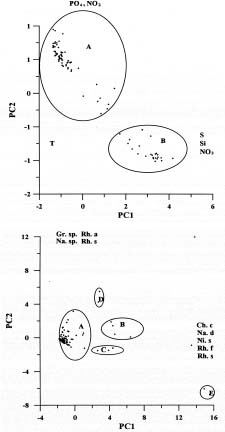
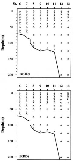
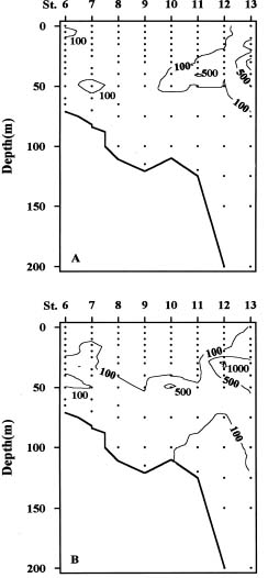
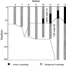
Abstract. Distributions of diatom assemblages in and around a persistent upwelling area off northeastern Taiwan were investigated during summer, 1994. Two water types and two diatom assemblages were defined by principal component analyses. The two water types represent the nutrient-depleted surface water and the nutrient-laden upwelled subsurface Kuroshio Water. During the period of this study, the latter water type did not outcrop but stayed in the subsurface layer, probably resulting from the outflowing of the warm nutrient-poor Taiwan Strait Water. Diatom assemblages indicated the interplay between the two water types. One assemblage, composed of cosmopolitan species in low density, represented the Background Assemblage, which was widely distributed in most of the surface water and also in the underlying upwelling water. The other assemblage, which was observed in the surface water in contact with the underlying upwelling water over the shelf break, represented an Enhanced Assemblage. Some species existing in the Background Assemblage were likely to be enhanced when they were brought into contact with the nutrient-rich upwelled subsurface Kuroshio Water and, subsequently, formed a new assemblage. When the water parcel containing the new assemblage flowed away from the nutrient-rich water, this Enhanced Assemblage sometimes switched back into the Background Assemblage a few days later.

Keywords: Background Assemblage; Diatom assemblage; East China Sea; Kuroshio; Upwelling.

Introduction

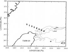
The Kuroshio Current originates from the sea east of the Philippines and flows northward along the east coast of Taiwan. When reaching the area off northeastern Taiwan, it is blocked by the East China Sea shelf and generates a cyclonic cold eddy over the shelf break (Chern and Wang, 1990; Tang, unpublished data). The cold water originates from upwelling of the Kuroshio subsurface Water (Liu et al., 1992a) provided by a counter-current over the continental slope landward of the impinging Kuroshio main stream (Chuang et al., 1993). This cold upwelling has been shown to persist throughout the year (Liu et al., 1992b) and constitutes one of the major nutrient inputs to the East China Sea (Wong et al., 1991; Gong et al., 1995). Outcropping of this upwelling water may be suppressed temporarily by the outflow of Taiwan Strait Water driven by the persistent southwesterly wind in summer (Gong et al., 1992). The residence time of water within the cold eddy has been estimated to be about a week (Liu et al., 1992b).

Light, temperature, nutrient supply, and zooplankton grazing have been recognized as the four most important factors affecting phytoplankton populations (Parsons et al.,

1984; Cullen et al., 1992). Studies of primary production in the southern East China Sea have been intense (Guo, 1991; Chen, 1992; Shiah et al., 1995, 1996); however, essential information regarding species composition of the phytoplankton assemblage in this area is rare. Guo (1991) reviewed the geographical distribution of the phytoplankton in the Philippine Sea, East China Sea, and the northwestern Pacific Ocean. Chen (1992) described a summer phytoplankton community structure in the upwelling area northeast of Taiwan. Possible controlling mechanisms on the distribution patterns of the diatom assemblage were discussed but not fully analyzed in these studies.

It is well recognized that physical and chemical driving forces in the ocean may have a strong impact on phytoplankton production, the growth rate (Shiah et al., 1995, 1996 and citations therein), and assemblage composition (Chiang and Taniguchi, 1993). The study of the spatial and temporal variability of the phytoplankton assemblage may serve as a useful indicator of the interactions among biological, physical, and chemical processes (Chiang et al., 1994 and citations therein). The complex hydrography observed in the East China Sea northeast of Taiwan suggested that such an area could be an ideal experimental ground to examine how physical and chemical processes affect the distribution patterns of phytoplankton assemblages. The study was performed in summer mainly for hydrographical reasons. As mentioned previously, during

⁴Corresponding author. Fax: (02) 462-1016.

Botanical Bulletin of Academia Sinica, Vol. 38, 1997

summer the upwelling of the cold and nutrient-rich Kuroshio subsurface Water may be suppressed by the outflow of the warm and oligotrophic Taiwan Strait Water. We expected to see a different diatom assemblage in the frontal zone of these two water masses from those within the water mass. We hypothesized that the spatial patchiness of the diatom assemblage observed in the study area might be a net result of physical (i.e. light availability), chemical (i. e. nutrient availability) and biological (i.e. grazing) interactions.

Materials and Methods

Sampling and Analysis

This study was conducted on Cruise 034 of R/V Ocean Researcher II in July, 1994. A total of eight sampling stations were occupied along a transect encompassing the inner and outer shelf of the southern East China Sea (Figure 1). Seawater was collected from a SeaBird CTD-General Oceanic Rosette assembly with 5-liter Go-Flo bottles. Temperature and salinity profiles were also recorded simultaneously. Light intensity was measured with a light meter (PAR sensor; QSP200L; Biospherical Inc.) installed on the research vessel. The depth of the euphotic zone was defined as 1% of the surface light penetrated.

liquid nitrogen. Nitrate was analyzed with a self-designed flow injection analyzer (Gong et al., 1992; Strickland and Parsons, 1972) and was reduced to nitrite with a cadmium wire activated with a copper sulfate solution. Phosphate and silicate were measured by the molybdenum blue and the silicomolybdenum blue method (Pai et al., 1990).

Data Analysis

Principal component analyses (PCAs) and cluster analyses (Pielou, 1984) were performed using the Statistical Analysis System (SAS). The PCAs were carried out with two data sets. The first data set (i.e. OD) included temperature, salinity, and four nutrients. The second data set (i.e. DD) was composed of twenty-two dominant diatom species. A dominant was defined as a species which appeared in more than 40% of samples that had been examined (Chiang and Taniguchi, 1993). The first principal component PC₁ and the second principal component PC₂ in the PCAs were used to identify subgroups by the average linkage clustering method (Euclidean distance = 1.0). Water types and diatom assemblages were defined by OD and DD, respectively.

Results

The T-S diagram (Figure 2) showed that temperature and salinity of water samples taken from the study area were in the ranges of 12_30°C and 34.00_34.70 psu, respectively. Temperature and salinity profiles suggested a two-layer structure along the sampling transect (Figures 3A and 3B). The water column could be characterized by a surface layer with higher temperature (> 26°C) and lower salinity (< 34.30 psu) and a subsurface layer of cooler and more saline water. An oblique front with temperature of 26°C and salinity of 34.30 psu could be clearly identified

Figure 1. Map of the East China Sea northeast of Taiwan showing sampling stations.

Diatom Species Composition

The method of microscopic examination of the diatom assemblages followed the method of Chiang and Taniguchi (1993). A 500 ml water sample was preserved by 25 ml of neutralized formalin. Identification and cell counts were made under a Nikon-TMD300 inverted microscope at 200× or 400×.

Nutrient Concentrations

Water samples were collected with clean 100 ml polypropylene bottles and were frozen immediately with

Figure 2. The T-S relationship of sea water along the sampling transect. Solid curve represents the mean T-S characteristic of the Kuroshio.

Chiang et al. — Spatial distribution of diatom species composition

between these two layers. At station 6, this front was located at 70_80 m and became more and more shallow when moved toward station 13 where its front depth was < 30 m. The nitrate distribution (Figure 3C) also portrayed such a two-layer structure. The 0.5 µM nitrocline followed almost exactly the same trend of the oblique front. Judging from the results shown in Figures 3A_C and research performed previously by Chern et al. (1990), Liu et al. (1992a), and others, we believed that this subsurface layer, with its high concentrations of nitrate and a dome-shaped structure in temperature and salinity, was the upwelled

subsurface Kuroshio Water, although it probably did not outcrop to the surface during the study period. On the other hand, the overlying nitrate-depleted surface layer with higher temperature and lower salinity probably was the Taiwan Strait Water, which had been driven by the persistent southwesterly winds and spread into the study area (Gong et al., 1992). Therefore, the front described here was a mixing zone of Taiwan Strait Water and the upwelled subsurface Kuroshio Water. The depth of the euphotic zone increased seaward (Figure 3C), with a value of 35 m at station 6 and 75 m at station 13.

Figure 3. Vertical profiles of temperature (A; °C), salinity (B; psu), nitrate concentrations (C; µM), phosphate concentrations (D; µM), dissolved silica concentrations (E; µM), diatom abundance (F; 10³ cells l^-1), and chlorophyll a concentrations (G; µg/l) along the sampling transect. Dashed line in (C) indicates euphotic depth.

Botanical Bulletin of Academia Sinica, Vol. 38, 1997

Table 1. Oceanographic data used as variables for the principle component analysis and their eigenvectors of PC₁ and PC₂. Percentage of variance explained is indicated below both PC₁ and PC₂.

Variables PC₁ (68.1%) PC₂ (27.7%)

Temperature -0.451 0.305

Salinity 0.424 -0.295

Dissolved Silica 0.474 -0.096

Phosphate 0.316 0.593

Nitrate 0.481 -0.092

Nitrite 0.244 0.671

The results derived from the PCAs on oceanographical data confirmed our speculation about the water masses. Table 1 showed that PC₁ explained 68.1% of the total variance and was positively correlated with salinity, dissolved silica, and nitrate but negatively correlated with temperature. PC₂ accounted for 27.7% of the total variance and positively correlated with phosphate and nitrite. In the scatter diagram of PC₂ on PC₁, two clusters (i.e. Cluster A and B) were clearly distinguished [Figure 4 (upper)]. Their depth distribution at all sampling stations was given in Figure 5A. Cluster A represented the Surface Water Type and was characterized with high temperature, low salinity, and low dissolved silica and nitrate concentrations. It appeared in the upper water column (i.e. < 40_75 m) of all stations. On the other hand, Cluster B represented the Upwelled Subsurface Water Type, located at the deeper area (i.e. > 40_75 m) of stations 8_13 but not observed at stations 6 and 7. This water type was characterized with low temperature, high salinity, and dissolved silica and nitrate concentrations.

Figure 3F_G showed that there was a high density patch of diatom abundance (i.e. > 10,000 cells l^-1) and chlorophyll a concentrations across the sampling transect. It appeared at the depth of 35_60 m at stations 10_13 and extended to the surface at station 13. Diatom abundance was low (i. e. < 5,000 cells l^-1) at the rest of the sampling area. When compared with the hydrography data, the upper boundary of this high density patch seemed coincident with the positions of the front (Figure 3A_B) and the nutricline (Figures 3C_E). The lower margin of this patch

Table 2. Twenty-two dominant diatom species, which occurred in more than 40% of samples, used as variables for the principle component analysis and their eigenvectors of PC₁ and PC₂. Percentage of variance explained is indicated below both PC₁ and PC₂.

Variables PC₁ (55.2%) PC₂ (15.8%)

Bacteriastrum comosum 0.222 -0.148

Cerataulina pelagica 0.226 0.189

Chaetoceros compressum 0.272 0.006

Chaetoceros lorenzianum 0.249 -0.147

Chaetoceros messanens 0.221 -0.219

Grammatophora sp. 0.090 0.387

Guinardia flaccida 0.249 - 0.182

Hemiaulus hauckii 0.247 0.126

Lauderia annulata 0.228 -0.234

Navicula distans 0.251 -0.089

Navicula sp. 0.119 0.355

Nitzschia closterium 0.220 -0.206

Nitzschia seriata 0.266 -0.044

Nitzschia sp. 0.118 0.055

Pseudoeunotia doliolus 0.168 -0.124

Rhizosolenia alata 0.179 0.349

Rhizosolenia fragilissima 0.253 0.174

Rhizosolenia imbricata 0.235 0.148

Rhizosolenia setigera 0.180 0.385

Rhizosolenia stolterfothii 0.263 0.040

Thalassionema nitzschioides 0.135 -0.235

Thalassiosira sp. 0.150 -0.209

Figure 4. Scatter diagram of PC₂ on PC₁ of the principal component analysis using oceanographic data (upper) and diatom species data (lower). Envelopes denote two clusters identified by an average cluster analysis.

Chiang et al. — Spatial distribution of diatom species composition

was located around the bottom of the euphotic zone, which ranged between 50_65 m from stations 10 to 13. These data strongly suggest that both light and nutrient (i.e. nitrate) availability might play crucial roles in determining the spatial pattern of diatom abundance along the sampling transect. A similar example of phytoplankton growth in a shelf-break front was reported by Marra et al. (1990)

Table 2 showed the results of PCAs on the diatom species data set. About 70% of the total variance could be explained by PC₁ and PC₂. The PC₁ was primarily influenced by Chaetoceros compressum, Navicula distans, Nitzschia seriata, Rhizosolenia fragilissima, and Rhizsolenia stolterfothii. The PC₂ was largely induced by Grammatophora sp., Navicula sp., Rhizosolenia alata, and Rhizosolenia setigera. Five clusters (i.e. Clusters A_E) were identified when PC₂ was plotted against PC₁ [Figure 4 (lower)]. Two diatom assemblages were well separated from these five Clusters. The Surface Assemblage was composed of Clusters B, C, D, E with the isolated Cluster # recorded at 40 m at station 11, and 15 m at station 13. Dominant species in this assemblage were Chaetoceros compressum, Chaetoceros lorenzianum, Nitzschia seriata, and Thalassionema nitzschioides (Table 3 and Figure 6A). Population density of the Surface Assemblage (1.0 × 10⁴ cells l^-1) was at least two times higher than that of the Background Assemblage (see below). The Surface Assemblage was found in the surface layer (< 75 m) at station 13 and subsurface layer (20_50 m) at stations 10_12 (Figure 5B). When compared with the distribution pattern of the water types (i.e. Clusters A and B), The Surface Assemblage was located at the transition zone (i.e. front) of the Surface Water Type (Cluster A) and the Upwelled Subsurface Water Type (Cluster B).

The Background Assemblage was represented by Cluster A and the isolated Cluster recorded at 25 m of station 11 [Figures 4 (lower) and 5B]. The neritic cosmopolitan Thalassionema nitzschioides was the major component of this assemblage (Table 3 and Figure 6B). With only one exception (5 m at station 6), population density of this assemblage was low and rarely exceeded 0.5 × 10⁴ cells l^-1. We noted that the Background Assemblage was distributed widely over the sampling area except for in the frontal zone (Figures 5B).

Summarizing all the results presented above, we found a very clear distribution pattern of the diatom assemblage along the sampling transect (Figure 7). The Surface Assemblage was characterized by a high population density (0.5_1.0 × 10⁴ cells l^-1) distributed only at the front where the warm, oligotrophic surface water met the cold, nutrient-rich upwelled Kuroshio subsurface Water. The rest of the sampling areas were dominated by Thalassionema nitzschioides, which constituted the major portion of the Background Assemblage.

Discussion

The structural properties of diatoms, either in terms of abundance (Figure 3F) or species composition (Figure 7)

Figure 5. Vertical distribution pattern of clusters derived from oceanographic data (A) and diatom species data (B).

Table 3. Distribution and some features of diatom assemblage defined by the principle component analysis in and around a upwelling sea area in the southern East China Sea.

Assemblage Surface Background

Diatom clusters B, C, D, E, # A, #

Distribution St. 10 (50) All the rest

(St. & depth) St. 11 (25_50)

St. 12 (20_40)

St. 13 (0_50)

Dominant species Chaetoceros compressum Thalassionema nitzschioides

Chaetoceros lorenzianum

Nitzschia seriata

Thalassionema nitzschioides

Botanical Bulletin of Academia Sinica, Vol. 38, 1997

Figure 7. Distribution of water types and diatom assemblage defined by principal component analysis along the sampling transect.

compared with the latter two water masses, the front was the only area where both light and nutrients (i.e. nitrate) were available simultaneously. Figure 3C clearly shows that the front was located above the bottom of the euphotic zone but below the 0.5 µM nitrocline. Dugdale (1976) has noted that for tropical oceanic phytoplankton, the typical values of the half-saturation constants (Ks) for nitrate uptake are 0.07 µM in oligotrophic environments and 0.98 µM in eutrophic environments. The Ks represent the concentrations at which nutrient uptake is half of its maximum value. Concentrations at the 2×Ks are associated with the maximum specific rate of nutrient uptake (Vm); therefore, concentrations below it have greatly reduced uptake rates, potentially enough to limit algal growth rates or biomass accumulation. In contrast, concentrations greater than the 2×Ks indicate that algal growth tends to be unconstrained by nutrient supply. In the same area, Shiah et al. (1995; 1996) showed that seasonal and spatial variability of phytoplankton photosynthetic performance (i.e. production and growth rates) were affected by light and nutrient supply. Our survey further indicated that these two environmental factors might also be crucial in determining the spatial patterns of phytoplankton (i.e. diatom) abundance and species composition.

With all the results derived from physical, chemical, and biological studies performed in this area, we propose the following scenario to explain the phenomenon we observed in this study. The Background Assemblage is probably widely distributed in the oligotrophic shelf water and the upwelled subsurface Kuroshio Water. When the Kuroshio current is blocked at the shelf break off northeastern Taiwan at a bottom depth > 200 m (Chern and Wang, 1990; Liu et al., 1992a, b) it then upwells to the surface (5 m d^-1) generating a cyclonic nutrient-rich cold

Figure 6. Vertical distribution of Nitzschia seriata, the dominant species of the Surface Assemblage (A; 10³ cells l^-1), and Thalassionema nitzschioides, the dominant species of the Surface Assemblage and Background Assemblage (B; 10³ cells l^-1).

were very patchy along the sampling transect. We believed the frontal zone, where the enhanced assemblage with high population density was located, must have had some unique physical and chemical characteristics to display such heterogeneity. Above and below the front were the oligotrophic surface water and the nutrient-rich upwelled subsurface water, respectively (Figures 3A_E; 5A). When

Chiang et al. — Spatial distribution of diatom species composition

eddy (Tang, unpublished data). During summer, the upwelled Kuroshio Subsurface Water is superimposed by, and then mixed with, Taiwan Strait Water driven by the southwesterly winds (Gong et al., 1992). In the subsurface Kuroshio Water, growth conditions (i.e. dark and cold) are unfavorable for the Background Assemblage. However, during its path to the surface, temperature turns warmer and light intensity (i.e. photosynthetic available radiance) becomes higher. Such amelioration of physical constraints plus proper nutrient supply have made some of the diatom species in the Background Assemblage grow prosperously (see Figure 6A) and then changed the old assemblage into a new one (i.e. the Enhanced Assemblage). This phenomenon and its driving mechanisms have been proposed by Ishizaka et al. (1986); Yamamoto et al. (1988); Hayward and Mantyla (1990), Marra et al. (1990), and Chiang et al. (1994).

Above the front, nutrients can be rapidly exhausted by the active growth of the Surface Assemblage which made the surface water a poor living environment. Shiah et al. (1996) demonstrated that the chlorophyll normalized production index (i.e. P^B_max) at the margin of the upwelling plume (P^B_max = 4.0 mgC mgChl^-1 h^-1) reduced dramatically when compared with the area adjacent to the center of the upwelling whose P^B_max value was two times higher. This nutrient deficient condition may decrease diatom abundance (i.e. biomass) and force the Enhanced Assemblage to switch back to the slowly growing Background Assemblage (Dodson and Thomas, 1977; Thomas et al., 1980; Ishizaka et al., 1983 and Chiang and Taniguchi, 1993). The same argument can explain why the Background Assemblage distributes all over the sampling area beneath the euphotic zone. There, light availability but not nutrient supply becomes the limiting factor restricting the development of the Background Assemblage into the Enhanced Assemblage.

Undoubtedly, zooplankton grazing must also play a strong role in regulating diatom abundance and thus species composition in the study area. Chen and Chen (1992) showed that zooplankton were also distributed unevenly in this area with a higher abundance recorded around the upwelling plume. In addition to the hypotheses proposed above, it is more reasonable to deduce that the low phytoplankton abundance observed at the upper water column outside the frontal zone is controlled by top-down (i.e. zooplankton grazing) and bottom-up (i.e. nutrient supply) forces, concurrently. Also of interest is that the chemical composition of zooplankton within the upwelling plume was different from that outside the plume (i.e. the coastal and Kuroshio Waters; Chen and Chen, 1992). Since diatom are a major food source for zooplankton in the open ocean (Chen and Chen, 1992), the species composition of the prey eventually will influence the chemical composition of their predators. This indicates that our results could be also very helpful in explaining the heterogeneous distribution pattern of zooplankton and of creatures at even higher trophic levels (i.e. larval and adult fishes) which prey on the zooplankton.

Conclusions

Both light and nutrient availability affect the spatial distribution pattern of the diatom assemblages in the upwelling area northeast of Taiwan. Outside the frontal zone the Background Assemblage occurs dominated by Thalassionema nitzschioides with low abundance. This assemblage is distributed widely in areas where either photosynthetic available radiance (the deep water) or nutrient supply (the surface water) are limited. In the region where living conditions become optimal, such as the frontal zone, where neither of the above factors are limiting, the old assemblage may transform into a new assemblage (i.e. the Enhanced Assemblage) dominated by different diatom species (Marshall and Nesius, 1996). After consulting the results of related studies performed in this area and also research conducted in other regions, we propose that the diatom species composition of the Background Assemblage and the Enhanced Assemblage might switch back and forth, depending on the growth conditions which are determined principally by the interactions of physical and chemical factors within and between water masses. Our study further points out that research into the distribution patterns of diatom assemblages is also very important in understanding the controlling mechanisms on zooplankton and fishery yield in this area.

Acknowledgments. We are grateful to Drs. K.-K. Liu and J. Chang for their constructive comments on this work. We also thank the officers and crews of R/V Ocean Researcher II. This study was supported by grants from the National Science Council, ROC. NSC83-0209-M-019-012K (K.-P. Chiang), NSC85-2611-M-002-005-K2 (F.-K. Shiah) and NSC-85-2611-M-019-014-K2 (G.-C. Gong).

Literature Cited

Chen, H. Y. and Y. L. L. Chen. 1992. Quantity and quality of summer surface net zooplankton in the Kuroshio current-induced upwelling northeast of Taiwan. Terrest. Atmosp. Ocean. Sci. 3: 321_334.

Chen, Y.L.L. 1992. Summer phytoplankton community structure in the Kuroshio Current-related upwelling northeast of Taiwan. Terrest. Atmosp. Ocean. Sci. 3: 305_320.

Chern, C.-S and J. Wang. 1990. On the mixing of waters at a northern offshore area of Taiwan. Terrest. Atmosp. Ocean. Sci. 1: 297_306.

Chern, C.-S., J. Wang, and D.-P. Wang. 1990. The exchange of Kuroshio and East China Sea shelf water. J. Geophys. Res. 95(C9): 16017_16023.

Chiang, K.-P. and A. Taniguchi. 1993. Formation of a diatom assemblage distributed widely in the North Pacific Polar Frontal Zone. Bull. Jap. Soc. Fish. Oceanogr. 57: 307_318.

Chiang, K.-P., A. Taniguchi, and S. Kato. 1994. Distribution of diatom assemblages in and around a warm core ring in the North Pacific Polar Frontal Zone. La mer 32: 195_207.

Chuang, W.-S., H. W. Li, T. Y. Tang, and C. K. Wu. 1993. Observation of the countercurrent on the inshore side of the Kuroshio northeast of Taiwan. J. Oceanogr. 49: 581_592.

Botanical Bulletin of Academia Sinica, Vol. 38, 1997

Cullen, J. J., X. Yang, and H. L. MacIntyre. 1992. Nutrient limitation of marine photosynthesis. In P. G. Falkowski and A. D. Woodhead (eds.), Primary productivity and biogeochemical cycles in the sea. N. Y., Plenum, pp. 69_88.

Dodson, A.N. and W.H. Thomas. 1977. Marine phytoplankton growth and survival under simulated upwelled and oligotrophic condition. J. Exp. Mar. Biol. Ecol. 26: 153_161.

Dugdale, D. C. 1976. Nutrient cycles. In D. Cushing and J. Walsh (eds.), The Ecology of the Sea, Blackwell, Oxford, pp. 141_172.

Fisher, T. R., L. W. Harding, D. W. Stanley, and L. G. Ward. 1988. Phytoplankton, nutrients, and turbidity in the Chesapeake, Delaware, and Hudson estuaries. Est. Coastal Shelf Sci. 27: 61_93.

Gong, G.-C., C.-Z. Shyu, W.-H. Shin, and K.-K Liu. 1992. Temperature fluctuation of the cold water off northern Taiwan: June-December, 1990. Acta Oceanogr. Taiwanica 28: 118_127.

Gong, G.-C., K.-K. Liu, and S.-C. Pai. 1995 Prediction of nitrate concentration from two end member mixing in the southern East China Sea. Continent. Shelf Res. 15(7): 827_842.

Guo, Y. J. 1991. The Kuroshio. Part II. Primary productivity and phytoplankton. Oceanogr. Mar. Biol. Annu. Rev. 29: 155_189.

Hayward, T.L. and A.W. Mantyla. 1990. Physcial, chemical and biological structure of a coastal eddy near Cape Mendocino. J. Mar. Res. 48: 825_850.

Ishizaka, J., M. Takahashi, and S. Ichimura. 1983. Evaluation of coastal upwelling effects on phytoplankton growth by simulated culture experiment. Mar. Biol. 76: 271_278.

Ishizaka, J., M. Takahashi, and S. Ichimura. 1986. Changes in the growth rate of phytoplankton in local upwelling around the Izu Peninsula, Japan. J. Plankton Res., 8(1): 169_181.

Liu, K.-K., G.-C. Gong, C.-Z. Shyu, S.-C. Pai, C.-L. Wei, and S.-Y. Chao. 1992a. Response of Kuroshio upwelling to the oneset of the northeast monsoon in the sea north of Taiwan: observation and numerical simulation, J. Geophys. Res. 97: 12511_12526.

Liu, K.-K., G.-C. Gong, S. Lin, C.-Z Shyu, C.-Y. Yang, C.-L. Wei, S.-C. Pai, and C. K. Wu. 1992b. The year-round up

welling at the shelf break near the northern tip of Taiwan as evidenced by chemical hydrography. Terrest. Atmosp. Ocean. Sci. 3: 234_276.

Marra, J., R. W. Houghton, and C. Garside. 1990. Phytoplankton growth at the shelf-break front in the Middle Atlantic Bight. J. Mar. Res. 48: 851_868.

Marshall, H. G. and K. K. Nesius. 1996. Phytoplankton composition in relation to primary production in Chesapeake Bay. Mar. Biol. 125: 611_617.

Pai, S.-C., C.-C. Yang, and J. P. Riley. 1990. Effects of acidity and molybdate concentration on the kinetics of the formation of the phosphoantimonyl molybdenum blue complex. Anal. Chim. Acta 229: 115_120.

Parsons, T. R., M. Takahashi, and B. Hargrave. 1984. Biological Oceanographic Processes. NY, Pergamon, 330 pp.

Pielou, E.C. 1984. The Interpretation of Ecological Data. John Wiely & Sons, New York, 263 pp.

Shiah, F.K., G.C. Gong, and K.K. Liu. 1995. A preliminary survey on primary productivity measured by the 14C assimilation method in the KEEP area. Acta Oceanogr. Taiwanica 34(1): 1_16.

Shiah, F.-K., G.-C. Gong, and K.-K. Liu. 1996. Light effects on phytoplankton photosynthetic performance in the southern East China Sea north of Taiwan. Bot. Bull. Acad. Sin. 37: 133_140.

Strickland, J.D.H. and T.R. Parsons. 1972. A practical handbook of sea water analysis. Fisheries Research Board of Canada, Bull., 167, Ottawa, 310 pp.

Thomas, W.H., M. Pollock, and D.L.R. Seibert. 1980. Effects of simulated upwelling and oligotrophy on chemostat-grown natural marine phytoplankton assemblages. J. Exp. Mar. Biol. Ecol. 45: 25_36.

Wong, G.T.F., S.-C. Pai, K.-K. Liu, C.-T. Liu, and C.-T.A. Chen. 1991. Variability of the chemical hydrography at the frontal region between the East China Sea and the Kuroshio northeast of Taiwan. Esturine, Coastal Shelf Sci. 33: 105_120.

Yamamoto, T., S. Nishizawa, and A. Taniguchi. 1988. Formation and retention mechanisms of phytoplankton peak abundance in the Kuroshio front. J. Plankton Res. 10: 1113_1130.