Bot. Bull. Acad. Sin. (2000) 41: 231-236

Chung — Spatial genetic structure in Hemerocallis

Spatial genetic structure in three populations of Hemerocallis hakuunensis (Liliaceae)

Myong Gi Chung

Department of Biology, Gyeongsang National University, Chinju 660-701, The Republic of Korea

(Received May 21, 1999; Accepted December 24, 1999)

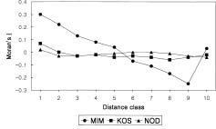
Abstract. Ninety-nine, 75, and 71 individuals were mapped and leaf samples were collected from three populations (10 × 15-m plot [MIM], 40 × 50-m plot [KOS], and 15 × 20-m plot [NOD]) of Hemerocallis hakuunensis to determine if spatial genetic structure existed in the three populations in terms of their ecological characteristics. A substantial spatial genetic structuring was found in MIM, whereas a weak structure was observed in NOD and KOS. Moran's I values were significantly different from the expected value (-0.010) in 137 (52.7%) of 260 cases in MIM, whereas significant Moran's I values were observed in 25 (10.4%) of 240 cases and 55 (20.4%) of 270 cases in NOD and KOS, respectively. The approximate minimum patch width also varied among the three populations: NOD = 3 m, MIM = 5 m, and KOS = 10 m. The differences in patch width may result from the differences in density, colonization history, thinning processes or any of a number of other factors among populations.

Keywords: Allozymes; Density; Hemerocallis hakuunensis; Moran's I; Spatial autocorrelation.

Introduction

During the past decade, spatial genetic structure has been quantified using spatial autocorrelation statistics using allozymes as genetic markers to understand the evolutionary dynamics of plant populations (e.g., Berg and Hamrick, 1995; Chung and Epperson, 1999; Dewey and Heywood, 1988; Epperson and Clegg, 1986; Perry and Knowles, 1991; Schnabel and Hamrick, 1990). These studies showed that individuals are not likely to be randomly distributed owing to factors such as limited seed and pollen dispersal, isolation in small patches, differential mortality, and microenvironmental selection. In addition to these factors, differences in density, pollinator behaviors, topography, and colonization history could result in a different genetic architecture in plant populations of a species (e.g., Chung et al., 1998; Knowles et al., 1992; Young and Merriam, 1994). All these aspects should be considered in studies of natural plant populations to gain insights into their maintenance mechanisms of genetic diversity.

Hemerocallis hakuunensis Nakai is commonly found in grasslands of mountainous areas, under pineoak forests on the hillsides, and under disturbed orchards of chestnut trees of the southern, central, and northwestern Korean Peninsula (Chung and Kang, 1994a). Individuals of the species have 5 to 16 flowers on the branched inflorescence. Flowers are orange-yellow and are usually visited by bees, bumblebees, and flies. They start to open before sunrise and remain open until the afternoon (Chung, pers. obs.). The species has no specialized mechanisms for seed dispersal (Chung, pers. obs.).

In this study, spatial autocorrelation using allozyme markers was conducted in three populations of H. hakuunensis to determine whether differences in spatial genetic structure existed in populations under different ecological conditions.

Materials and Methods

In August 1995 and August 1997, 99, 75, and 71 individuals were mapped and leaf samples were collected within a 10 × 15-m plot (Mich'eon-myeon, Chinju-shi, Prov. Gyeongsangnam-do, hereafter referred to as MIM), a 40 × 50-m plot (Sangri-myeon, Kosung-gun, Prov. Gyeongsangnam-do, hereafter referred to as KOS), and a 15 × 20-m plot (Nogodan, Mts. Chiri, Prov. Chollanam-do, hereafter referred to as NOD), respectively. Ecological characteristics of the three populations are summarized in Table 1. Leaf samples were placed in plastic bags wrapped with a wet paper towel and stored on ice to prevent protein denaturation prior to returning to the laboratory, where they were stored at 4°C until protein extraction.

Leaf samples were cut finely, and crushed with a mortar and pestle. A phosphatepolyvinylpyrrolidone extraction buffer (Mitton et al., 1979) was added to the leaf samples to facilitate crushing and to aid enzyme stabilization. The cellular extract was absorbed onto 4 × 6-mm Whatman 3MM chromatography paper wicks, which were then stored at -70°C until needed. Electrophoresis was performed using 11% starch gels. Fourteen putative loci were resolved from eight enzyme systems using three gel/electrode buffer combinations. Two Poulik buffer systems were used: a modification (Haufler, 1985) of Soltis et al. (1983) "system 6" was used to resolve leucine aminopeptidase (LAP), fluorescent esterase (FE) and a modi

Fax: +82-591-754-0086; E-mail: mgchung@nongae.gsnu.ac.kr

Botanical Bulletin of Academia Sinica, Vol. 41, 2000

fication (electrode buffer of pH 8.6) of Haufler (1985) resolved diaphorase (DIA), alcohol dehydrogenase (ADH), and b-galactosidase (b-GAL). A morpholine citrate buffer system, a modification (Chung and Kang, 1994b) of that of Clayton and Tretiak (1972), was used to resolve malate dehydrogenase (MDH), phosphoglucoisomerase (PGI), and 6phosphogluconate dehydrogenase (6PGD). Stain recipes were taken from Soltis et al. (1983), except for the DIA and b-Gal, which were taken from Cheliak and Pitel (1984). The genetic basis of enzyme banding patterns was inferred from observed segregation patterns in light of typical subunit structure and subcellular compartmentalization (Weeden and Wendel, 1989). Putative loci were designated sequentially, with the most anodally migrating isozyme designated `1', the next `2', etc. Likewise, alleles were designated sequentially with the most anodally migrating allele designated `a'.

Lap2, Dia-2, and Pgd2 were not included in this study due to faint or inconsistent staining. Pgi-1 and b-Gal were monomorphic in all individuals. Moran's I, a spatial autocorrelation index, is a spatially weighted product-moment correlation coefficient in which neighboring individuals are compared in terms of their deviation from the mean of all observations. For spatial autocorrelation analysis, the genotypic data were coded so that allele frequency values of 1.0, 0.5, or 0.0 were assigned to individuals being homozygous for a given allele, heterozygous for that allele or genotypes with no copies of that allele, respectively, for each polymorphic locus (Sokal and Oden, 1978). Only one allele was considered at a dialellic locus, because the second allele contributes identical information. For a locus having more than two alleles, all alleles at that locus, regardless of their frequencies, were used for the spatial analysis. However, alleles that were presented by less than five copies (frequencies <2.6%, <3.3%, and <3.5% in MIM, KOS, and NOD, respectively) were excluded as non-informative for spatial analysis. Every possible pair of individuals was considered as a join (a connection between two individuals) and was assigned to one of ten distance classes. Because measures of small-scale autocorrelation more accurately represent the spatial structure, the first of ten distance classes was designed based on an estimate of the average distance which separates nearest neighbor

individuals (see Tables 1-3). Moran's I values (Sokal and Oden, 1978) were calculated for each of ten distance classes by interpopulational distance classes. Each I value was used to test significant deviations from the expected values, E(I) = -1/(N-1) (Cliff and Ord, 1981). A significant positive value of Moran's I indicates that the neighboring individuals have more alleles in common than would be expected by chance, whereas a significant negative value suggests that distant individuals have fewer alleles in common. Overall significance of each correlogram, and hence the presence of spatial structure, for each allele was tested using Bonferroni's criterion (Sakai and Oden, 1983). All calculations and statistical analyses were performed using the SAAP program (ver. 4.3) written by D. Wartenberg.

Results

According to the criteria above, 26 (MIM and KOS) and 24 alleles (NOD) were used for spatial autocorrelation analysis. The spatial autocorrelation coefficients, Moran's I, for the three populations are presented in Tables 2 through 4. For population MIM, Moran's I values were significantly different from the expected value (-0.010) in 137 (52.7%) of 260 cases, and the overall correlogram was significant for 19 (73%) of 26 alleles (Table 2). For distance classes 1 to 5 (0 < 5 m), 68 statistically significant positive values were observed and eight significant negative values were detected. This indicates that individuals are genetically similar when separated by 5 m or less. For population KOS, somewhat weaker spatial genetic structure was observed (Table 3). Moran's I values were significantly different from the expected value (-0.013) in 55 (20.4%) of 270 cases, and the overall correlogram was significant for 10 (37%) of 27 alleles (Table 3). For distance classes 1 and 2 (0 < 9 m), 15 significantly positive values were found, but no significant negative value was observed within the distance classes. For population NOD, a considerably weak spatial genetic structuring was found (Table 4). Moran's I values were significantly different from the expected value (-0.014) in 25 (10.4%) of 240 cases, and the overall correlogram was significant for only four (16.7%) of 24 alleles (Table 4). For distance classes 1 and 2 (0 < 4 m), only three significant positive values were ob

Table 1. Ecological characteristics of Hemerocallis hakuunensis examined.

Population code Sample size Elevation (m) Plot area (m²) Population size Density Habitat

MIM 97 340 150 Several thousands 0.64 Recently established, 3% hillslopes, understory in chestnut tree orchard, Hemerocallis hakuunensis is dominant.

KOS 75 240 2,000 <100 0.04 Undisturbed, 15% hillsides, understory of dense pine-oak forests.

NOD 71 1,350 300 Several thousands 0.24 Undisturbed, open grasslands with Hosta capitata (Liliaceae) and other herbs, H. hakuunensis is abundant.

Chung — Spatial genetic structure in Hemerocallis

Table 2. Spatial autocorrelation coefficients (Moran's I) over ten distance classes for 26 alleles in population MIM of Hemerocallis hakuunensis. The expected E(I) = -0.010.

Distance class (upper distance bound, m)

Allele 1(1) 2(2) 3(3) 4(4) 5(5) 6(6) 7(9) 8(10) 9(12) 10(14) P¹ Allele frequency

Adh^d 0.06 0.03 -0.04 -0.02 -0.08* -0.04 0.03* -0.02 -0.03 0.07 0.230 0.076

Adh^e 0.12* 0.22** 0.14** 0.05 0.06* -0.10* -0.15** -0.04 -0.04 0.11 0.000 0.308

Adh^g 0.21** 0.03 -0.08* 0.17** 0.01 -0.06 -0.04 -0.02 -0.14** -0.54* 0.000 0.611

Dia1^c 0.27** -0.04 -0.06 0.07* -0.09* -0.02 0.01 0.01 -0.14** -0.33 0.000 0.330

Dia1^e 0.15** 0.03 -0.04 -0.04 -0.01 0.03 0.02 -0.11* -0.25** 0.81** 0.000 0.595

Dia1^g 0.23** 0.17** 0.15** 0.17** 0.03 -0.06 -0.13** -0.19** -0.24** 0.36* 0.000 0.040

Fe1^e 0.00 0.05 0.01 0.00 -0.09* 0.01 0.01 -0.01 -0.15** -0.05 0.027 0.084

Fe1^g 0.80** 0.64** 0.46** 0.30** 0.18** -0.14** -0.32** -0.62** -0.76** 0.20 0.000 0.738

Fe1ⁱ 0.13* 0.12** -0.07 -0.13** -0.12** 0.01 0.06** -0.06 -0.08 -0.01 0.007 0.121

Fe2^c 0.66** 0.55** 0.35** 0.27** 0.11** -0.23** -0.32** -0.28** -0.35** 0.14 0.000 0.676

Fe2^e 0.41** 0.28** 0.29** 0.25** 0.08** -0.09* -0.24** -0.21** -0.34** 0.23 0.000 0.152

Fe2^g -0.02 -0.00 0.03 -0.05 -0.00 -0.03 -0.01 -0.05 0.03 0.26 1.000 0.121

Lap1^c 0.80** 0.68** 0.42** 0.25** 0.18** -0.15** -0.39** -0.57** -0.43** 0.26 0.000 0.954

Mdh^d 0.65** 0.51** 0.46** 0.24** 0.18** -0.19** -0.28** -0.43** -0.70** -0.17 0.000 0.919

Pgd1^c 0.16** 0.09* -0.02 -0.02 -0.00 -0.08* -0.04 0.03 -0.00 0.11 0.047 0.801

Pgd1^f 0.49** 0.54** 0.21** 0.15** 0.14** -0.11** -0.22** -0.39** -0.48** 0.10 0.000 0.066

Pgd1^g 0.04 -0.02 -0.04 -0.02 0.03 -0.06 -0.00 0.07 -0.10* 0.17 0.428 0.122

Pgi2^d 0.00 -0.00 -0.03 -0.02 0.05 -0.03 0.00 -0.12* -0.01 0.11 0.204 0.052

Pgi2^g 0.67** 0.42** 0.37** 0.27** 0.01 -0.11** -0.13** -0.61** -0.84** -0.16 0.000 0.805

Pgi2ⁱ 0.61** 0.42** 0.27** 0.13** 0.00 -0.10** -0.15** -0.36** -0.56** 0.24 0.000 0.052

Pgi2^k 0.06 0.04 -0.06 0.07* -0.01 -0.07 -0.01 -0.04 -0.04 -0.12 0.347 0.038

Pgi3^a 0.05 0.05 0.01 -0.07 -0.02 0.02 -0.03 -0.00 -0.04 0.04 0.761 0.081

Pgi3^c 0.10* 0.10* -0.08* -0.03 -0.09* 0.01 0.04** -0.07 -0.16** 0.17 0.017 0.237

Pgi3^e 0.49** 0.33** 0.18** 0.02 0.14** -0.08* -0.24** -0.17** -0.10* -0.03 0.000 0.581

Pgi3^g 0.52** 0.30** 0.20** 0.09* 0.12** -0.08* -0.20** -0.22** -0.35** -0.29 0.000 0.066

Pgi3ⁱ 0.03 0.07* -0.07 -0.08* -0.01 0.00 -0.03 0.03 0.09* -0.49* 0.106 0.035

Average 0.30 0.22 0.13 0.08 0.04 -0.07 -0.11 -0.17 -0.25 0.03

¹Overall correlogram significance (Bonferroni approximation). ^* = P < 0.05; ^** = P < 0.01.

Table 3. Spatial autocorrelation coefficients (Moran's I) over ten distance classes for 27 alleles in population KOS of Hemerocallis hakuunensis. The expected E(I) = -0.013.

Distance class (upper distance bound, m)

Allele 1(1) 2(2) 3(3) 4(4) 5(5) 6(6) 7(9) 8(10) 9(12) 10(14) P¹ Allele frequency

Adh^b 0.14** -0.05 -0.01 -0.05 0.07 -0.14** -0.29** 0.03 -0.00 -0.03 0.003 0.247

Adh^d 0.15** 0.00 0.01 -0.03 0.03 -0.13** -0.33** -0.22** -0.05 0.08* 0.001 0.700

Adh^e 0.44** 0.06 0.09** 0.09* 0.06 0.10** -0.04 -0.63** -0.58** -0.35** 0.000 0.053

Dia1^a 0.08** 0.05 -0.11** -0.07 -0.05 0.01 -0.01 0.07 -0.11* 0.01 0.037 0.047

Dia1^b 0.16** -0.08 -0.13** 0.05 0.01 -0.04 -0.07 -0.09 -0.10 0.10* 0.001 0.437

Dia1^d 0.12** -0.08 -0.05 0.02 0.03 -0.11* -0.15 -0.06 -0.02 0.06 0.018 0.520

Fe1^b 0.03 -0.02 -0.01 -0.06 -0.03 -0.04 -0.03 0.04 -0.05 0.00 1.000 0.887

Fe1^c 0.03 -0.01 -0.05 -0.08 -0.00 -0.00 -0.02 0.02 -0.04 0.01 1.000 0.107

Fe2^a 0.09** -0.02 -0.05 -0.11 -0.03 -0.01 -0.02 0.08 -0.11* 0.01 0.098 0.840

Fe2^b 0.03 -0.01 -0.05 -0.08 -0.00 -0.00 -0.02 0.02 -0.04 0.01 1.000 0.107

Fe2^c 0.12** -0.04 -0.02 -0.08 -0.06 -0.03 -0.01 0.12* -0.16** -0.00 0.013 0.053

Lap1^a -0.02 -0.01 -0.03 0.00 -0.00 -0.04 0.01 -0.05 0.01 0.01 1.000 0.213

Lap1^b -0.05 0.07* -0.02 -0.05 -0.04 -0.03 0.11 -0.07 0.02 -0.01 0.255 0.707

Lap1^c -0.04 0.05 -0.00 -0.05 -0.09* -0.03 0.15* -0.04 0.01 -0.02 0.187 0.080

Mdh^a 0.04 0.00 0.00 -0.02 -0.06 -0.04 -0.15* -0.08 0.11** -0.07 0.060 0.040

Mdh^b 0.09* 0.05 -0.01 0.04 -0.09 -0.17** -0.25** -0.03 0.06 -0.01 0.003 0.913

Mdh^c -0.01 0.01 -0.02 0.09* -0.09 -0.06 -0.10 0.01 -0.05 0.04 0.216 0.040

Pgd-1^b 0.23** 0.13** -0.05 -0.19** -0.35** -0.04 0.30** -0.34** 0.15** -0.03 0.000 0.733

Pgd-1^c 0.20** 0.09** -0.04 -0.09 -0.39** -0.10* 0.24** -0.11 0.05 0.02 0.000 0.227

Pgd-1^d 0.02 0.01 -0.01 -0.02 0.03 0.04 0.03 -0.13* -0.07 -0.08 0.173 0.040

Pgi2^b -0.00 0.09* -0.09* 0.12** -0.07 -0.09* 0.03 -0.06 -0.03 0.02 0.100 0.040

Pgi2^e -0.02 -0.05 -0.02 -0.02 -0.01 0.04 -0.08 0.04 -0.06 0.02 1.000 0.840

Pgi2^h -0.04 -0.03 0.07* -0.06 -0.06 0.01 -0.15 -0.01 -0.03 0.02 0.212 0.067

Pgi3^c -0.02 -0.00 0.02 0.02 -0.02 0.05 -0.06 -0.10 -0.06 -0.05 0.812 0.460

Pgi3^e -0.02 -0.03 -0.07 -0.01 0.08* 0.01 -0.09 -0.00 0.03 -0.03 0.444 0.180

Pgi3^f -0.01 -0.05 0.01 0.06 -0.03 -0.02 -0.07 -0.07 0.02 -0.01 1.000 0.087

Pgi3^g -0.01 -0.02 -0.06 -0.04 0.03 0.02 0.03 -0.07 0.06 -0.03 0.979 0.207

Average 0.07 0.00 -0.03 -0.02 -0.04 -0.03 -0.04 -0.06 -0.04 -0.02

¹Overall correlogram significance (Bonferroni approximation). ^* = P < 0.05; ^** = P < 0.01.

Botanical Bulletin of Academia Sinica, Vol. 41, 2000

Table 4. Spatial autocorrelation coefficients (Moran's I) over ten distance classes for 24 alleles in population NOD of Hemerocallis hakuunensis. The expected E(I) = -0.014.

Distance class (upper distance bound, m)

Allele 1(1) 2(2) 3(3) 4(4) 5(5) 6(6) 7(9) 8(10) 9(12) 10(14) P¹ Allele frequency

Adh^a 0.02 0.05 -0.07 -0.18** 0.02 -0.04 0.00 -0.03 0.02 -0.02 0.047 0.082

Adh^b 0.07* 0.06 -0.06 0.01 0.10** -0.06 -0.10 -0.15* -0.16** -0.27** 0.003 0.253

Adh^d 0.09* 0.06 -0.09 -0.06 0.05* 0.03 -0.07 -0.13* -0.13* -0.22* 0.168 0.664

Dia1^a -0.01 -0.04 -0.06 0.04 0.01 -0.00 -0.11* 0.07 -0.02 0.05 0.360 0.061

Dia1^b -0.01 -0.01 0.05 -0.06 -0.00 -0.05 -0.03 0.02 0.02 0.00 1.000 0.267

Dia1^d 0.03 0.01 -0.07 -0.01 -0.02 -0.03 -0.06 0.05 -0.03 0.10 0.578 0.480

Dia1^e 0.01 -0.06 -0.08 -0.13* 0.03 0.01 -0.05 0.01 0.01 -0.02 0.458 0.192

Fe1^b 0.04 -0.08 -0.07 -0.01 -0.08* 0.04 0.15** 0.03 -0.09 -0.07 0.018 0.897

Fe2^a 0.01 -0.08 -0.09 0.05 -0.03 -0.00 0.08 0.03 -0.06 -0.16 0.503 0.767

Fe2^b 0.04 -0.08 -0.07 -0.01 -0.08* 0.04 0.15** 0.03 -0.09 -0.07 0.018 0.103

Fe2^c 0.03 -0.08 -0.14* -0.02 0.01 0.03 0.06 -0.01 -0.04 -0.07 0.341 0.130

Lap1^a 0.02 -0.01 0.04 -0.06 -0.01 0.03 0.02 -0.05 0.01 -0.06 1.000 0.185

Lap1^b 0.02 -0.05 0.01 0.03 -0.04 -0.03 0.09* -0.13* 0.03 -0.06 0.300 0.610

Lap1^c 0.02 -0.02 0.04 0.06 -0.04 -0.02 0.05 -0.05 0.00 0.02 0.960 0.205

Lap2^a 0.04 -0.08 -0.01 0.09 -0.01 -0.02 -0.03 0.02 -0.06 0.05 0.544 0.069

Lap2^b 0.01 -0.11 -0.02 0.07 -0.00 -0.01 -0.04 -0.06 -0.01 0.08 0.792 0.911

Mdh^b 0.02 -0.04 0.00 -0.09 0.04* -0.05 -0.06 0.09* -0.10 -0.07 0.341 0.720

Pgd1^b 0.04 0.08 -0.05 0.01 -0.04 0.02 -0.00 0.04 -0.02 0.03 0.909 0.863

Pgi2^a 0.02 0.02 0.07 -0.08 -0.04 0.06 -0.07 0.06 -0.13* 0.02 0.290 0.226

Pgi2^c 0.07* -0.11 0.00 -0.01 -0.06 -0.07 -0.01 -0.02 0.13** -0.13 0.069 0.048

Pgi2^d 0.02 -0.05 0.16** -0.10 -0.04 0.06 -0.05 0.02 -0.08 -0.07 0.069 0.658

Pgi2^f -0.01 -0.04 -0.09 -0.08 0.02 0.03 -0.05 -0.02 0.05 -0.07 1.000 0.069

Pgi3^a -0.02 -0.08 -0.02 0.08 -0.01 -0.02 0.01 -0.08 -0.02 0.08 0.771 0.315

Pgi3^c -0.03 -0.08 -0.05 0.11* -0.01 0.03 -0.02 -0.03 -0.01 0.05 0.351 0.678

Average 0.02 -0.03 -0.03 -0.02 -0.01 -0.00 -0.00 -0.01 -0.03 -0.04

¹Overall correlogram significance (Bonferroni approximation). ^* = P < 0.05; ^** = P < 0.01.

served at a scale of 3 m. A relatively higher mean Moran's I value in the first distance class was observed in MIM (0.30) than in KOS (0.07) or NOD (0.02).

The distance at which the mean Moran's I value first intersects the E(I) value may represent the shortest length of an irregularly shaped patch size (Sokal, 1979). The approximate minimum patch width also was varied among the three populations: MIM of 5 m, KOS of 10 m, and NOD of 3 m (Figure 1).

Discussion

The ratio of significant I values in populations of H. hakuunensis was higher than predicted by a 5% type I error, indicating that genetic structuring within populations existed for the three populations. The mean correlogram of a population of H. hakuunensis indicates that the minimum patch width was approximately 3-10 m. The level of genetic relatedness seen among nearby individuals in these sites could easily be explained by localized seed dispersal.

The number of significant I values and the average Moran's I values for each distance class indicates that population MIM is more structured than populations KOS and NOD. Factors possibly contributing to the different levels of genetic substructuring include differences in density, topography, colonization history, or any of a number of others (Hamrick and Nason, 1996; J. L. Hamrick, pers. comm.). The area occupied by population MIM was cleared to plant chestnut trees about 20 years ago (J. S. Park, a landowner, pers. comm.). It is highly likely that

Figure 1. Correlograms for populations MIM, KOS, and NOD using mean values of Moran's I and 10 distance intervals. Distance classes in meters as in Tables 2 to 4.

Population MIM was established by a few seed sources from adjacent areas, and the size of the population has been rapidly increasing due to sufficient resources (i.e., fertilizers) and low interspecific competition. A larger population size of H. hakuunensis was observed in an orchard of chestnut trees compared to populations found in an understory of pine forests and forest margins. More limited pollinator flight distance in a dense young population under chestnut trees, coupled with limited seed dispersal may be factors for shaping a strong spatial genetic substructuring in MIM. In contrast, population NOD is located on undisturbed, high elevation, relatively open grasslands in which H. hakuunensis is abundant (several thousands individuals are scattered over the grasslands)

Chung — Spatial genetic structure in Hemerocallis

with Hosta capitata (Liliaceae) and other herbs. In this habitat, the pollinator flight range would be relatively long, resulting in a relatively large neighborhood size. An intermediate degree of genetic structuring was observed in KOS. Only 75 individuals were recorded in a 20 × 50 m area of dense pine forests with other shrubs such as oaks and sumacs. Under such a dense forest, the pollinator flight distance would be restricted. The age of the oldest Pinus densiflora was 68 years old in KOS, suggesting no fire had occurred during the past several decades.

Hemerocallis hakuunensis has no specialized mechanisms for seed dispersal (ovate 5 mm long seed), and many seedlings are found near maternal plants in natural populations (Chung, pers. obs.). Since gene movement in seed plants is a sequential (two-step process via pollen then by seed), observed genetic structure may be most strongly influenced by limited seed dispersal compared to pollen movement. Even with long distance pollen flow, limited seed movement can result in patches of halfsibs (Hamrick and Nason, 1996). In other words, the male gamete moves twice, but the female gamete only moves via seed. Thus, family structure can result solely by limited seed dispersal. Considering this argument, the considerably weaker genetic substructuring found in NOD and KOS compared with that of MIM also suggests that the thinning process between the seedling and adult stages does away with most of the genetic structure in populations NOD and KOS, if interspecific competitions with other herbs is strong. The greater density of MIM might indicate less thinning of new recruits, which could explain the higher relatedness values seen in this site.

It may be of interest to compare the present results with a previous study of another outcrossing liliaceous plant which has a similar life history and ecological traits with the Hemerocallis species. Maki and Masuda (1994) examined spatial genetic structure using the same computer program as in this study in two outcrossing populations (10 × 20-m and 2 × 20-m areas) of Chinographis japonica var. japonica. The variety, occurring in the understory of forests in western Japan, is a self-incompatible perennial. As with H. hakuunensis, bees visit the flowers and no specialized mechanism of seed dispersal is known (Maki and Masuda, 1994). The pattern of overall correlogram found in C. japonica var. japonica (Moran's I values were significant in 15 [23%] and [27%] of 66 cases in two populations) is similar to those of H. hakuunensis, parIn summary, the approximate minimum patch width in the populations of H. hakuunensis examined is 3-10 m, indicating that populations are structured on a small scale. This study describes in detail several features of the fine-scale population genetic structure, which may result from the differences in density, colonization history, thinning processes or a number of other factors.

Acknowledgments. We thank Drs. J. L. Hamrick, B. K. Epperson, and Eric Myers for comments on the earlier version of the manuscript. This research was supported in part by a Korea Science and Engineering Foundation grant (971-0505-029-2) to MGC.

Literature Cited

Berg, E. and J.L. Hamrick. 1995. Fine-scale genetic structure of a turkey oak forest. Evolution 49: 110-120.

Cheliak, W.M. and J.P. Pitel. 1984. Technique for Starch Gel Electrophoresis of Enzyme from Forest Tree Species. Agric. Canada Forest Serv., Petawawa Nat. Forest Inst., Inform. Rep. PI-X-42.

Chung, M.G. and S.S. Kang. 1994a. Morphometric analysis of the genus Hemerocallis L. (Liliaceae) in Korea. J. Plant Res. 107: 165-175.

Chung, M.G. and S.S. Kang. 1994b. Genetic variation and population structure in Korean populations of Eurya japonica (Theaceae). Am. J. Bot. 81: 1077-1082.

Chung, M.Y., G.M. Chung, M.G. Chung, and B.K. Epperson. 1998. Spatial genetic structure in populations of Cymbidium goeringii (Orchidaceae). Genes Genet. Syst. 73: 281-285.

Chung, M.G. and B.K. Epperson. 1999. Spatial genetic structure of clonal and sexual reproduction in a populations of Adenophora grandiflora (Campanulaceae). Evolution 53: 1068-1078.

Clayton, J.W. and D.N. Tretiak. 1972. Amine-citrate buffers for pH control in starch gel electrophoresis. J. Fish. Res. Board Can. 29: 1169-1172.

Cliff, A.D. and J.K. Ord. 1981. Spatial Processes-Methods and Applications. Pion Limited, London.

Dewey, S.E. and J.S. Heywood. 1988. Spatial autocorrelation in a population of Psychotria nervosa. I. Distribution of genotypes. Evolution 47: 834-838.

Epperson, B.K. and M.T. Clegg. 1986. Spatial autocorrelation of flower color polymorphisms within substructured populations of morning glory (Ipomoea purpurea). Am. Natl. 128: 840-858.

Hamrick, J.L. and J.D. Nason. 1996. Consequences of dispersal in plants. In O. E. Rhodes, R. K. Chesser and M. H. Smith (eds.), Population Dynamics in Ecological Space and Time. University of Chicago Press, Chicago, IL., pp. 203-236.

Haufler, C.H. 1985. Enzyme variability and modes of evolution in Bommeria (Pteridaceae). Syst. Bot. 10: 92-104.

Knowles, P., D.J. Perry, and H.A. Foster. 1992. Spatial genetic structure in two tamarack [Larix laricina (Du Roi) K. Koch] populations with differing establishment histories. Evolution 46: 572-576.

Maki, M. and M. Masuda. 1994. Spatial genetic structure within two populations of a self-incompatible perennial, Chinographis japonica var. japonica (Liliaceae). J. Plant Res. 107: 283-287.

Mitton, J.B., Y.B. Linhart, K.B. Strugen, and J.L. Hamrick. 1979. Allozyme polymorphisms detected in mature needle tissue of ponderosa pine. J. Hered. 70: 86-89.

Perry, D.J. and P. Knowles. 1991. Spatial genetic structure within sugar maple (Acer saccharum Marsh.) stands. Heredity 66: 137-142.

Sakai, A.K. and N.L. Oden. 1983. Spatial pattern of sex expression in silver maple (Acer saccharium L.): Morista's index and spatial autocorrelation. Am. Natl. 122: 489-508.

Schnabel, A. and J.L. Hamrick. 1990. Comparative analysis of population genetic structure in Quercus macrocarpa and Q. gambelii (Fagaceae). Syst. Bot. 15: 240-251.

Sokal, R.R. 1979. Ecological parameters inferred from spatial

Botanical Bulletin of Academia Sinica, Vol. 41, 2000

correlograms. In G. P. Patil and M. L. Rosenzweig (eds.), Contemporary Quantitative Ecology and Related Ecometrics. International Cooperative Publishing House, Fairland, pp. 167-196.

Sokal, R.R. and N.L. Oden. 1978. Spatial autocorrelation in biology. 1. Methodology. Biol. J. Linn. Soc. 10: 199-249.

Soltis, D.E., C.H. Haufler, D.C. Darrow, and G.J. Gastony. 1983. Starch gel electrophoresis of ferns: a complication of grinding buffers, gel and electrode buffers, and staining

schedules. Am. Fern J. 73: 9-27.

Weeden, N.N. and J.F. Wendel. 1989. Genetics of plant isozymes. In D.E. Soltis and P.S. Soltis (eds.), Isozymes in Plant Biology. Dioscorides Press, Portland, OR., pp. 46-72.

Young, A.G. and H.G. Merriam. 1994. Effects of forest fragmentation on the spatial genetic structure of Acer saccharum Marsh. (sugar maple) populations. Heredity 72: 201-208.

Hemerocallis hakuunensis (Liliaceae) ¤TºØ±Ú¸s¤§°ò¦]ºc³yªº

¦a°ì¤À§G

M.G. Chung

Department of Biology, Gyeongsang National University

Chinju 660-701, The Republic of Korea

¤À§O¨Ó¦Û Hemerocallis hakuunensis ¤§¤TºØ±Ú¸s¡A§Y [MIM]¡B[KOS] ¤Î [NOD] ªº 99¡B75 ©M 71 ­ÓÅé³Q©w¦ì¥B¦¬¶°¨ä¸­¸Õ¼Ë¥H±Àºâ¬O§_±q¨ä¥ÍºA¯S©Ê¤§°Ñ¼Æ¥i¬Ý¥X¦¹¤T±Ú¸s¤§°ò¦]ºc³yªº¦a°ì¤À§G¡C±q MIM ¥iµo²{¬Û·íµ{«×¤§°ò¦]ºc³yªº¦a°ì¤À§G¡A¦ý NOD ¤Î KOS ªÌ«h¸û®z¡C¦b MIM ¤§ 260 ­Ó®×¨Ò¤¤¦³ 137 ­Ó (¦û 52.7%) ¨ä Moran's I ­È©M´Á±æ­È (-0.010) ¦³ÅãµÛ¤£¦P¡A NOD 240 ­Ó®×¨Ò¤¤¤§ 25 ­Ó (¦û 10.4%)¡AKOS 270 ­Ó®×¨Ò¤¤¤§ 55 ­Ó (¦û 20.4%) ¦³ÅãµÛ¤§ Moran's I ­È¡C²Ê¦ô¤§ minimum patch width ¦b¤T±Ú¸s¤]¤£¦P¡A§Y¡G NOD = 3 m¡AMIM = 5 m ¤Î KOS = 10 m¡C¦¹ patch width ¤§®t²§¥i¯à¬O±K«×¡A´Ï ¦aÁc´Þ¾ú¥v¡A®ø´î¹Lµ{©Î­Y¤z¨ä¥L¦]¤l¦b¤T±Ú¸s¶¡¤§¤£¦P©Ò¾É­P¡C

ÃöÁäµü¡G ²§ºc²¡¡F±K«×¡FHemerocallis hakuunensis¡FMoran's I¡F¦a°ì¦Û¬ÛÃö¡C